The monthly data releases this week showed that consumer, producer, and commodity inflation were all abating. All three were now running within .1% of 2.7% YoY. Commodity prices, which had rising at as high a rate as 11% YoY last July, were declining fastest. The first consumer confidence reading for April came in a little light.
This week the high frequency weekly indicators strongly contradicted one another. Let's start with the biggest negatives.
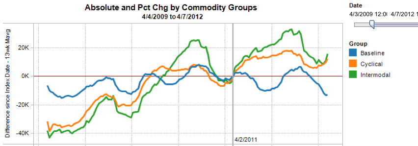
Rail traffic remained negative, and this week there was no good rationalization.
The American Association of Railroads reported a 4% decline in traffic YoY, or -20,200 cars. This week could not be blamed on coal, as even without coal, overall traffic edged up by a mere 800 cars, or +0.2% YoY. Intermodal traffic was up 2500 carloads, or +1.1%, but other carloads decreased -22,600, or -7.7% YoY. Railfax's graph of YoY traffic remained positive but deteriorated further this week. Oddly, Railfax's data shows that all of the decline is in "baseline" materials; rail hauling of cyclically sensitive materials remains in strong improvement.
Employment related indicators were strongly contradictory:
The Department of Labor reported that Initial jobless claims surged 23,000 to 380,000 last week, the highest report since January, mirroring the big increase in the first week of April one year ago. The four week average also rose by 6750 to 368,500.
The Daily Treasury Statement showed that for the first 9 days of April, $65.0 B was collected vs. $65.5 B a year ago, an absolute decline. In the last 20 reporting days, however (a more valid measure), $141.7 B was collected vs. $121.9 B a year ago, an increase of $19.8 B, or +16.2%!
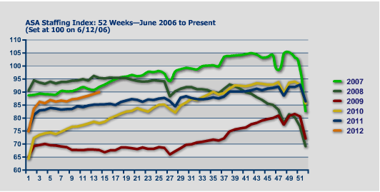
The American Staffing Association Index rose again by one to 90. It is now rising quickly, and is very close to its pre-recession readings of 2007. Should it continue at this pace, it will reach an all time high by June sometime.
Housing reports had a generally positive week:
The Mortgage Bankers' Association reported that the seasonally adjusted Purchase Index decreased -0.5% from the prior week, but was up a strong +5.5% YoY. The Refinance Index decreased another -3.8% from the previous week. Because the MBA's index was substituted for the Federal Reserve Bank's weekly H8 report of real estate loans in ECRI's WLI, I've begun comparing the two. This week for the second week in a row, and for the first time in four years real estate loans held at commercial banks were up, +0.2% on a YoY basis. On a seasonally adjusted basis, these bottomed in December and are now up +1.3% .
YoY weekly median asking house prices from 54 metropolitan areas at Housing Tracker were up +3.8% from a year ago. This number peaked at over +4% in February, but has now remained positive for 4 1/2 months. Via Calculated Risk, we are told that the NAR is likely to report a 3% YoY increase in median home sale prices for March. We should know by sometime this summer whether the Case-Shiller index follows the upward turn in the other indexes.
Sales were once again surprisingly positive.
Gasoline prices were flat at $3.94, the first week in months that there was not any increase. Oil was down slightly at $102.83. Both of these remain above the point where they can be expected to exert a constricting influence on the economy. Gasoline usage, at 8681 M gallons vs. 9181 M a year ago, was off -5.4%. The 4 week moving average is off -4.0%. These are among the best comparisons in months.
Turning now to high frequency indicators for the global economy:
The TED spread fell .02 to 0.380. This index remians slightly below its 2010 peak, generally steady for the last 7 weeks, and has declined from its 3 year peak of 3 months ago. The one month LIBOR declined .001 to 0.240. It is well below its 12 month peak set 3 months ago, remains below its 2010 peak, and has returned to its typical background reading of the last 3 years.
The Baltic Dry Index at 972 was up 44 from 928 one week ago, and up 302 from its 52 week low, although still well off its October 52 week high of 2173. The Harpex Shipping Index was flat at 395 in the last week.
Finally, the JoC ECRI industrial commodities index fell from 124.26 to 123.74. It has resumed its fade, at a pace about equal to April one year ago. This indicator appears to have more value as a measure of the global economy than the US economy.
This week we got some strongly contradictory signals from our high frequency indicators. Rail traffic, initial claims, industrial commodity prices and credit spreads all showed weakness. Three of these happen to be components of ECRI's WLI, so it is no surprise that it fell last week, although its 6 month growth metric continued to be more positive.
On the other hand, withholding taxes, temporary staffing, sales, housing, and money supply are all positive, some strongly so. Several of these are also leading indicators.
My best guess is that we are replaying last year, where seasonal increases in gasoline prices in the first part of the year cause the Oil choke collar to tighten, and weaknesses to appear in a number of indexes. I suspect this weakness will last until about midyear, and lead to the same double-dippism we heard in 2010 and 2011. This year might even be slightly worse. The weakness will cause the Oil choke collar to loosen, and the economy will become "surprisingly strong" as we head towards the end of the year.
Employment related indicators were strongly contradictory:
The Department of Labor reported that Initial jobless claims surged 23,000 to 380,000 last week, the highest report since January, mirroring the big increase in the first week of April one year ago. The four week average also rose by 6750 to 368,500.
The Daily Treasury Statement showed that for the first 9 days of April, $65.0 B was collected vs. $65.5 B a year ago, an absolute decline. In the last 20 reporting days, however (a more valid measure), $141.7 B was collected vs. $121.9 B a year ago, an increase of $19.8 B, or +16.2%!
The American Staffing Association Index rose again by one to 90. It is now rising quickly, and is very close to its pre-recession readings of 2007. Should it continue at this pace, it will reach an all time high by June sometime.
Housing reports had a generally positive week:
The Mortgage Bankers' Association reported that the seasonally adjusted Purchase Index decreased -0.5% from the prior week, but was up a strong +5.5% YoY. The Refinance Index decreased another -3.8% from the previous week. Because the MBA's index was substituted for the Federal Reserve Bank's weekly H8 report of real estate loans in ECRI's WLI, I've begun comparing the two. This week for the second week in a row, and for the first time in four years real estate loans held at commercial banks were up, +0.2% on a YoY basis. On a seasonally adjusted basis, these bottomed in December and are now up +1.3% .
YoY weekly median asking house prices from 54 metropolitan areas at Housing Tracker were up +3.8% from a year ago. This number peaked at over +4% in February, but has now remained positive for 4 1/2 months. Via Calculated Risk, we are told that the NAR is likely to report a 3% YoY increase in median home sale prices for March. We should know by sometime this summer whether the Case-Shiller index follows the upward turn in the other indexes.
Sales were once again surprisingly positive.
The ICSC reported that same store sales for the week ending April 7 rose +0.9% w/w, and also rose +4.5% YoY. Johnson Redbook reported a 4.1% YoY gain. Shoppertrak reported a whopping 20.7% YoY gain having everything to do with the timing of Easter. The 14 day average of Gallup daily consumer spending remained high at $76, $10 above the equivalent period last year.
Money supply was also positive:
M1 rose +1.1% last week, and was also up +0.8% month over month. On a YoY basis it declined slightly to +17.5%, so Real M1 is up 15.1%. YoY. M2 was up +2.2% for the week, and also up +0.5% month over month. Its YoY advance fell slightly to +9.8%, so Real M2 was up 7.2%. Real money supply indicators continue slightly less strongly positive on a YoY basis, although not so much as in previous months. It has resumed rising slightly on a month over month basis.
Bond prices were mixed and credit spreads widened slightly:
Weekly BAA commercial bond rates rose +.04% t0 5.29%. Yields on 10 year treasury bonds fell +.06% to 2.21%. The credit spread between the two, which had a 52 week maximum difference of 3.34% in October, rose slightly again to 3.07%. There has been a very slight weakening in this measure in the last two weeks.
The energy choke collar remains engaged:
Gasoline prices were flat at $3.94, the first week in months that there was not any increase. Oil was down slightly at $102.83. Both of these remain above the point where they can be expected to exert a constricting influence on the economy. Gasoline usage, at 8681 M gallons vs. 9181 M a year ago, was off -5.4%. The 4 week moving average is off -4.0%. These are among the best comparisons in months.
Turning now to high frequency indicators for the global economy:
The TED spread fell .02 to 0.380. This index remians slightly below its 2010 peak, generally steady for the last 7 weeks, and has declined from its 3 year peak of 3 months ago. The one month LIBOR declined .001 to 0.240. It is well below its 12 month peak set 3 months ago, remains below its 2010 peak, and has returned to its typical background reading of the last 3 years.
The Baltic Dry Index at 972 was up 44 from 928 one week ago, and up 302 from its 52 week low, although still well off its October 52 week high of 2173. The Harpex Shipping Index was flat at 395 in the last week.
Finally, the JoC ECRI industrial commodities index fell from 124.26 to 123.74. It has resumed its fade, at a pace about equal to April one year ago. This indicator appears to have more value as a measure of the global economy than the US economy.
This week we got some strongly contradictory signals from our high frequency indicators. Rail traffic, initial claims, industrial commodity prices and credit spreads all showed weakness. Three of these happen to be components of ECRI's WLI, so it is no surprise that it fell last week, although its 6 month growth metric continued to be more positive.
On the other hand, withholding taxes, temporary staffing, sales, housing, and money supply are all positive, some strongly so. Several of these are also leading indicators.
My best guess is that we are replaying last year, where seasonal increases in gasoline prices in the first part of the year cause the Oil choke collar to tighten, and weaknesses to appear in a number of indexes. I suspect this weakness will last until about midyear, and lead to the same double-dippism we heard in 2010 and 2011. This year might even be slightly worse. The weakness will cause the Oil choke collar to loosen, and the economy will become "surprisingly strong" as we head towards the end of the year.